In light of the recent
escalation of US tariff policy,
see also [1], this is my short write up of an Econ 101 take on tariffs,
just as a reasonable baseline for thinking about who actually pays for the them.
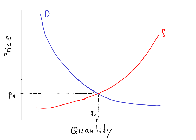
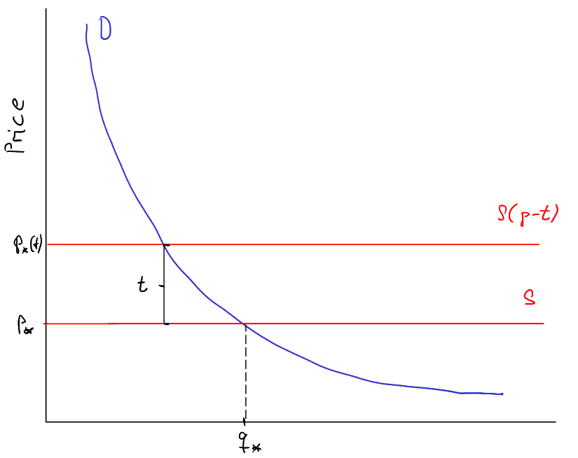
The model considers a simplified market, let's say the US market, in which an importer
demands a quantity \( D(p) \) of a foreign good at a market price \( p \).
This good is provided by a foreign supplier who is willing to supply \( S(p) \) units at
market price \( p \).
Assuming that supply \( S(p) \) is increasing in \( p \) and demand \( D(p) \) is decreasing
in \( p \), there is a unique price-quantity pair \( (p_{*}, q_{*}) \) at which supply equals
demand
\begin{align}
S(p) = D(p) \qquad \qquad \text{(Market equilibrium condition).}
\end{align}
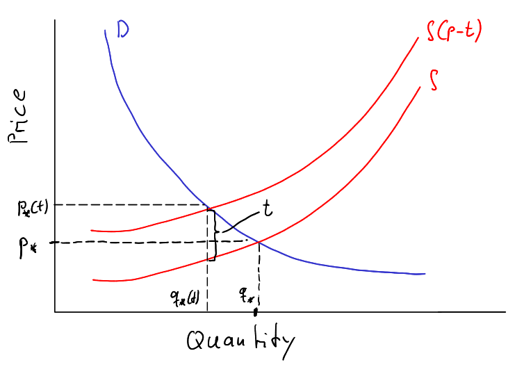
A tariff of \( t \ge 0 \) per unit that has to be paid by the supplier now acts as a tax and
yields the shifted curve \( S(p - t) \), since at the market price \( p \), the supplier will
only receive a revenue of \( p - t \) per unit.
Interestingly, the shift in equilibrium market price \( p_{*}(t) - p_{*} \) seems to be larger
than \( 0 \) but smaller than \( t \) meaning that the supplier passes some of the tariff
through to the importer.
Using some calculus, we can compute the exact derivative (in the simple model) of the
equilibrium price with respect to the tariff.
Define the function \( F(t, p): = S(p - t) - D(p) \), which satisfies
\begin{align}
F(0, p_{*}) = 0
\qquad \text{ and } \qquad
\partial_{p} F(t, p) = S'(p - t) - D'(p) > 0.
\end{align}
Assuming that supply and demand are sufficiently smooth, the
implicit function theorem
yields that the tariff-price pairs in market equilibrium \( (t, p_{*}(t)) \), which are just the zeros of \( F \), can be parameterized in \( t \) via a differentiable equilibrium price function \( p_{*}(t) \) with derivative
\begin{align}
p_{*}'(t)
& =
\frac{-\partial_{t} F(t, p_{*}'(t))}{\partial_{p} F(t, p_{*}'(t))}
=
\frac{S'(p_{*}(t) - t)}{S'(p_{*}(t) - t) - D'(p_{*}(t))}
=
\Big( 1 - \frac{D'(p_{*}(t))}{S'(p_{*}(t) - t)} \Big)^{-1}
\in
[0, 1]
\end{align}
At \( t = 0 \), the derivative is therefore given by \( ( 1 - D'(p_{*}) / S'(p_{*}) )^{-1} \).
The ratio of the derivatives can also be expressed as as the ratio of demand and supply
elasticities
\begin{align}
\frac{D'(p_{*})}{S'(p_{*})}
=
\frac{ D'(p_{*}) \cdot p_{*} / q_{*} }{ S'(p_{*}) \cdot p_{*} / q_{*} }.
=
\frac{ D'(p_{*}) \cdot p_{*} / D(p_{*})}{S'(p_{*}) \cdot p_{*} / S(p_{*})}.
\end{align}
The derivative of the equilibrium price therefore depends on how reactive supply and demand
are with respect to price changes.
Obligatory reference to The Wire whenever elasticities are mentioned.
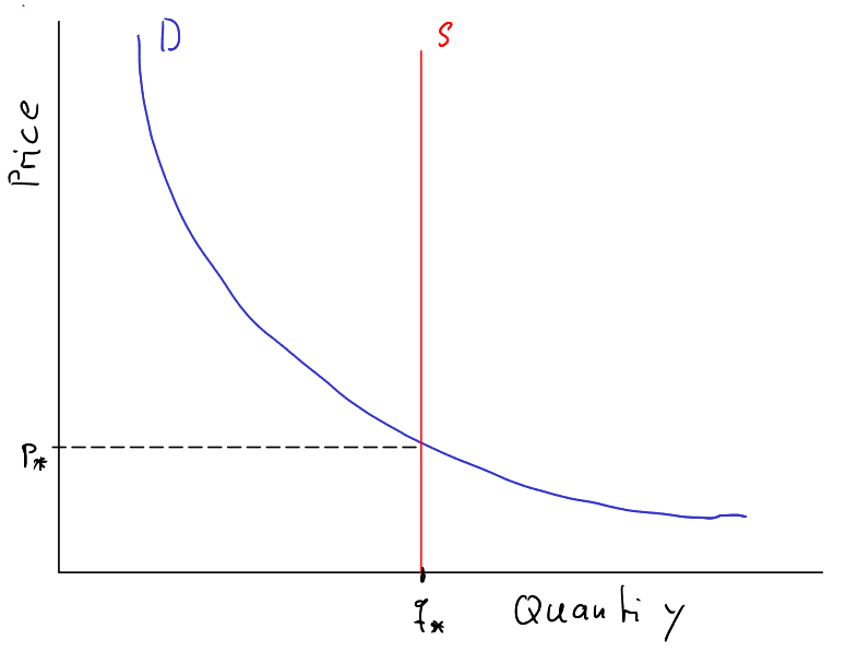
When supply is perfectly inelastic, i.e., constant in \( p \), the supplier is willing
provide the same quantity for any price.
In this setting, the shifted supply curve is identical to the non-shifted curve, the
derivative of the market price goes to zero and the price itself stays constant.
This means that the tariff is paid completely by the supplier.
The reverse happens when supply is perfectly elastic and its derivative goes to infinity.
In this setting, the derivative of the market price goes to \( 1 \) andshifting the supply
curve changes the price by \( t \).
This means that the tariff is paid completely by the importer.
The calculations can also be done for a percentage tariff but we then lose the nice
interpretation of the shifting curves.
For \( \tau \in [0, 1] \) and an imposed tariff of \( \tau \cdot 100\% \) the adjusted
supply is given by \( S((1 - \tau) p) \).
Analogously, we then define \( F(\tau, p): = S((1 - \tau) p) - D(p) \) with
\begin{align}
\partial_{p} F(\tau, p) = (1 - \tau) S'((1 - \tau) p) - D'(p) > 0.
\end{align}
The same reasoning as before then yields the existence of a function \( p_{*}(\tau) \)
that gives the equilibrium price at tariff \( \tau \) with derivative
\begin{align}
p_{*}'(\tau)
& =
\frac{- \partial_{\tau} F(\tau, p_{*}(\tau))}
{\partial_{p} F(\tau, p_{*}(\tau))}
=
\frac{ p_{*}(\tau) S'((1 - \tau) p_{*}(\tau)) }
{ (1 - \tau) S'((1 - \tau) p_{*}(\tau)) - D'(p_{*}(\tau))}
\end{align}
At \( \tau = 0 \), this evaluates to \( p_{*}'(0) = p_{*} (1 - D'(p_{*}) / S'(p_{*}) )^{-1} \),
which now includes the proportionality with respect to the price.
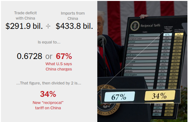
Surprisingly, this very simple model, is already enough to derive the Trump administration
tariff formula, see [2].
Assuming for simplicity that imports as demand in equilibrium \( D(p_{*}(\tau)) \) is
measured in real dollars, the change of imports with respect to the tariff at \( \tau = 0 \)
is
\begin{align}
\frac{d}{d \tau} D(p_{*}(\tau)) \Big|_{\tau = 0}
& =
D'(p_{*}) p_{*}'(0)
=
D'(p_{*}) \frac{p_{*}}{D(p_{*})} \frac{p_{*}'(0)}{p_{*}} D(p_{*})
=
\varepsilon \varphi D(p_{*}),
\end{align}
where \( \varepsilon = D'(p_{*}) p_{*} / D(p_{*}) \) is the import elasticiy with respect to
price and \( \varphi = p_{*}'(0) / p_{*} \) is the pass-trough rate of the tariff.
To a first order approximation, the change in imports is then
\begin{align}
D(p_{*}(\tau)) - D(p_{*}) \approx \varepsilon \varphi D(p_{*}) \tau
\end{align}
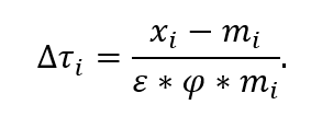
Setting this change equal the difference of real exports and imports, in order to induce a trade
balance of zero, yields the formula
\begin{align}
\tau
\approx
\frac{ X - D(p_{*}) }{ \varepsilon \varphi D(p_{*}) },
\end{align}
where \( X \) are US exports, which are not part of the model but exogenously taken as given.
(In terms of the Trump formula, \( m_{i} = D(p_{*}) \), \( x_{i} = X \) and
\( \Delta \tau_{i} = \tau \) because we have assumed an initial tariff of zero in the model)
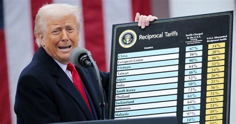
The office of the US trade representative then
(conveniently?)
estimate \( \varepsilon \approx -4 \) (in [2], it says \( \varepsilon \approx 4 \) but
that's the wrong sign, since the import elasticity has to be negative) and
\( \varphi \approx 1/4 \) to arrive at the
reciprocal tariff
(left side of poster) and then half it (right side of poster) or impose at least a tariff of
\( 10\% \), see [3] and [4].